Practical exercises on OpenCV
The following exercises aim to give you hands-on experience with some common computer vision algorithms. OpenCV is perhaps the most popular library for computer vision tasks, as it provides optimised implementations of many common computer vision algorithms. This work was created by Christian Richardt and Tadas Baltrušaitis in spring 2012.
Getting started
Unfortunately, it is not trivial to install OpenCV and the first few steps are always quite tricky – particularly using the C or C++ interfaces. However, the new Python bindings (introduced in OpenCV 2.3) are more accessible and thus used in the following exercises. To spare you the installation effort, we have prepared a fully-functional virtual machine based on Ubuntu. The virtual machine (1.1 GB zipped) can be opened with the free VirtualBox software on most operating systems (tested on Windows 7 and Mac OS X 10.7).
On the virtual machine, you can use gedit (Texteditor) for editing your Python scripts with syntax highlighting, and python {filename}.py in a terminal to run your code. You can also experiment with the interactive Python shell ipython, which can run scripts using the %run script.pycommand.
We encourage you to use the provided virtual machine for solving the exercises. However, if you know what you are doing, you are welcome to install OpenCV (2.3 or higher) with Python bindings yourself.
The OpenCV and NumPy documentations will come in handy while solving the exercises.
1. Convolution [25]
To get started, first download the script week1.py. It provides function stubs for the four exercises below which it feeds with a test image and convolution kernel. Useful functions for this supervision include np.zeros_like and cv2.copyMakeBorder.
- Implement basic convolution by translating the C code on page 26 of the lecture notes to Python. The function
basic_convolutionshould return the result as an image with the same size and datatype as the input image. You can assume that kernels are normalised, so the term/(mend*nend)should be left out. Please also include a progress indicator that prints to the console iffverboseis true. [8] - Improve your implementation from the previous exercise by first centering the filtered image inside the black border and then filling the black border. This can be done by conceptually extending the input image by replicating the edge pixels of the image (‘clamp-to-edge’). [5]
- Now apply the convolution theorem to speed up convolution. A good starting point for your own implementation is the
convolveDFTfunction in the documentation of OpenCV’s dft function. [9] - Finally extend your previous implementation to produce the same result as exercise 2 (centred result with clamp-to-edge border treatment).[3]
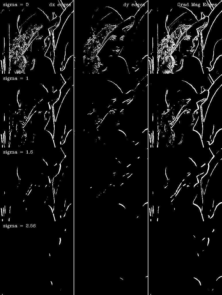
2. Edge detection [15]
To get started, first download the script week2.py. It provides function stubs for the helper functions you will need for the exercises, together with the code for loading and storing required images. The input image is already smoothed and subsampled using pyrDown function, this is to supress some of the noise. Be careful about the input and output types of the library functions you will use as some of them expect floating point numbers at 32 or 64 bit precision whilst others take in 8 bit integers, be sure to read their documentation carefully.
-
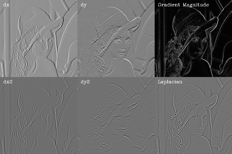
- Using convolution with appropriate kernels calculate the approximations of the first and second-order partial derivatives:
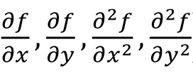
the magnitude of the Gradient
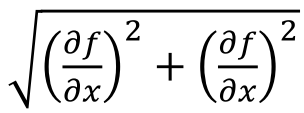
and the Laplacian (∇2)
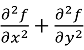
of the input image. A stub function for this exercise isComputeGradients. [6] - Extract the edges from the first-order partial derivatives and the gradient magnitude images using amplitude thresholding. A stub function for this exercise is
ComputeEdges. For this you can use the OpenCV functionthreshold(note that the function expects theCV_32Ftype). As a threshold value use 0.075. [2] - Locating zero-crossing in a 2D image is non-trivial, so instead we will use the Canny edge detector. Experiment with the OpenCV Canny edge detection function with various threshold values. A stub function for this exercise is
ComputeCanny. [2]
Your results should look like combinedGradients.png (for part a) and combinedEdges.png (for parts b and c).
- Using convolution with appropriate kernels calculate the approximations of the first and second-order partial derivatives:
- Create a scale-space representation of the input image with sigma values of 1, 1.6, and 2.56. A stub function for this exercise is
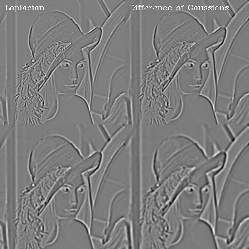
scaleSpaceEdges, which will use your previously completedComputeGradientsandComputeEdgesfunctions to calculate the edges of the resulting images. You will find the OpenCV functionGaussianBluruseful. Your result should look like scaleSpace.png. [2] - Using the previously calculated Gaussians, compute the Differences of Gaussians:
Gs=1.6 * I – Gs=1 * I and Gs=2.56 * I – Gs=1.6 * I.
Next, calculate the Laplacians of the Gaussians with sigmas 1 and 1.6:
∇2(Gs=1 * I) and ∇2(Gs=1.6 * I)
How is the Difference of Gaussians related to the Laplacian of Gaussian? You might find the OpenCV functionLaplacianuseful. [3]
Your result should look like laplacianVsDoG.png.
3. Panorama stitching [15]
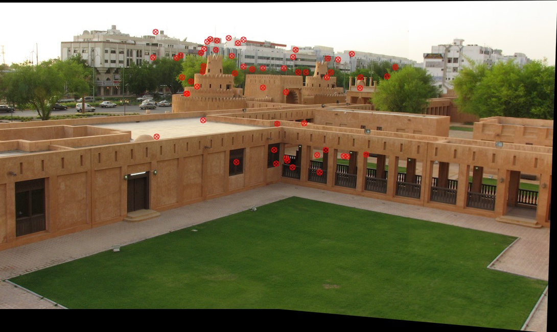
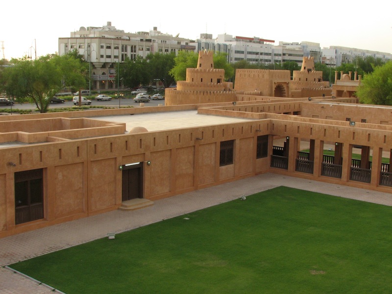
In these exercises, you will build your own basic panorama stitcher which will align and combine two images into one panorama (more details on this process). This is achieved by extracting features in both images, finding corresponding features between the two images to calculate the transform between images and finally warping them to combine them into one image, which should look like this: panorama.jpg.
To get started, first download this week’s script week3.py and the two images you will be using as input: Image1.jpg and Image2.jpg. The script provides functions for all the main steps involved in panorama stitching. The sections of the code you need to complete are indicated with ‘TODO’.
- The first step in panorama stitching is to extract features from both input images. Features are localised at a ‘keypoint’ and described by a ‘descriptor’. In the
extract_featuresfunction, use SURF to detect features and extract feature descriptors. Ensure thatdescriptorsis returned as an array of size n × 64. [4] - The
find_correspondencesfunction finds features with similar descriptors usingmatch_flann, which uses a kd-tree for efficient correspondence matching.match_flannreturns an array with two columns (one for each image), in which each row lists the indices of corresponding features in the two images. Convert this into two arrays,points1andpoints2, which give the coordinates of corresponding keypoints in corresponding rows.These correspondences are visualised in the filecorrespondences.jpg(created by the script) and which should look like this:correspondences.jpg. [2] - Next, you need to work out the optimal image size and offset of the combined panorama. For this, you’ll need to consider the positions of each images’ corners after the images are aligned. This can be calculated using the homogeneous 2D transform (3×3-matrix) stored in ‘
homography’. From this, you can calculate the totalsizeof the panorama as well as theoffsetof the first image relative to the top-left corner of the stitched panorama. If you get stuck, please skip this exercise and move to the next one. [5] - Now combine the two images into one panorama using the
warpPerspectivefunction. On top of the panorama, please draw the features that were used to estimate the transform between the images usingdrawChessboardCorners(withpatternWasFound=False). The resultingpanorama.jpgimage should look like this: panorama.jpg. [4]
4. Naïve Bayes for machine learning [15]
In this exercise, you will use a Normal Bayes Classifier to build your own optical character recognition (OCR) system. The classifier assumes that feature vectors from each class are normally distributed, although not necessarily independently (so covariances are used instead of simple variances). This is a slightly more advanced version of a Naive Bayes Classifier. During the training step, the classifier works out the means and covariances of the distribution for each class (in our case letters) in addition to the prior probabilities of each class. In the prediction step, the classifier uses the Bayes rule to work out the probability of the letter belonging to each of the classes (combining the likelihood with prior).
To get started, first download this week’s script week4.py and the two data sets you will be using (taken fromhttp://www.seas.upenn.edu/~taskar/ocr/). The smaller data set contains only 2 letters and the larger one containing 10 – a more challenging task. The data is split in such a way that two thirds of the images are used for training the classifier and the remaining third for testing it. The loading of data and spliting into training and test partitions is already done for you in the provided code.
You will be using an already cleaned up dataset containing 8×16 pixel binary images of letters. Examples of letters you would be recognising are ![]()
![]()
![]() . Every sample is loaded into an array
. Every sample is loaded into an array trainSamples(2|10) and testSamples(2|10), with every row representing an image (layed out in memory row-by-row, i.e. 16×8=128). This results in a 128-dimensional feature vector of pixel values. The ground truth (actual letters represented by the pixels) are in trainResponses(2|10), testResponses(2|10), for each of the data sets.
The sections of the code you need to complete are indicated with ‘TODO’.
- The first step in supervised machine learning is the training of a classifier. It can then be used to label unseen data. For this you will need to finish the
CallNaiveBayesmethod. Use theNormalBayesClassifierclass for this. The training, response and testing data are already layed out in the format expected by the classifier. [5] - Once we have a classifier, it is important to understand how good it is at the task. One way to do this for multi-way classifiers is by looking at the confusion matrix. The confusion matrix lets you know what object are being misclassified as each other, and gives you ideas of what additional features to add. Another useful evaluation metric is the average F1 score for each of the classes. These have already been written for you, and the code will report these statistics for the classifier you use. You can see that the performance on a-vs-b classification is much better than that of 10 letters. [0]
- Currently we are using the pixel values directly for the character recognition. Come up with additional features to improve the classification accuracy, such as say height and width, or even a number of contours – feel free to experiment. Just concatenate features as new columns to the data or replace some of the less informative existing pixels by the new features. Add your modifications to the feature vectors using the stub function
PreprocessData, and this will be used by the classifier; examples of how to iterate over the data are shown in this method. Be careful as theNormalBayesClassifierexpects training data to be in floating-point format. [10]